Table of contents
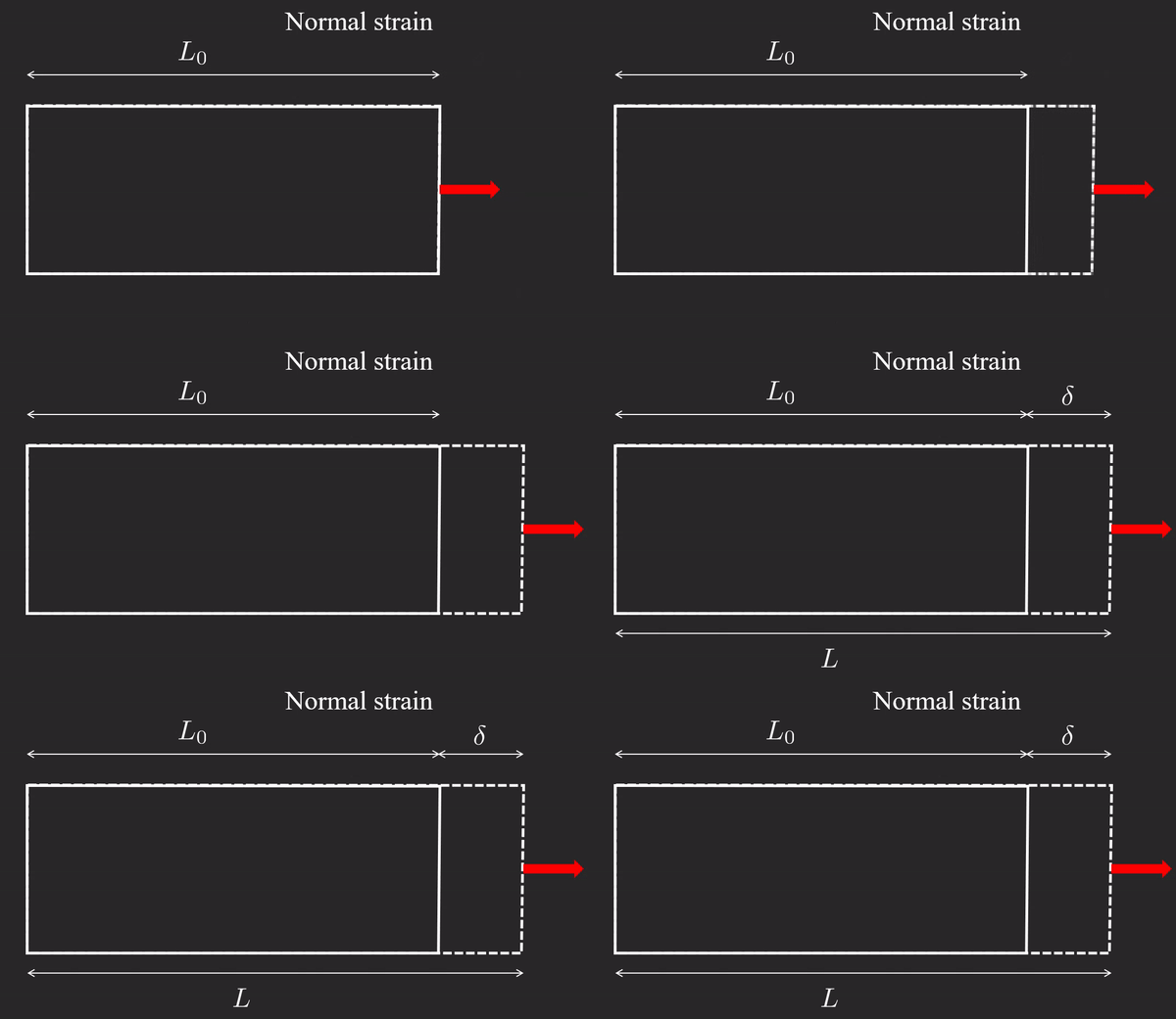
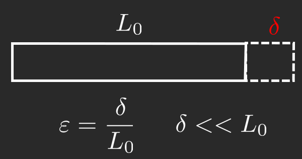
ε : = L − L 0 L 0 = δ L 0 \boxed{\varepsilon :=\dfrac{L-L_0 }{L_0 }=\dfrac{\delta }{L_0 }} ε := L 0 L − L 0 = L 0 δ where δ \delta δ deformation and ε \varepsilon ε engineering strain , or linear strain . This definition only holds under the assumption δ < < L \delta << L δ << L
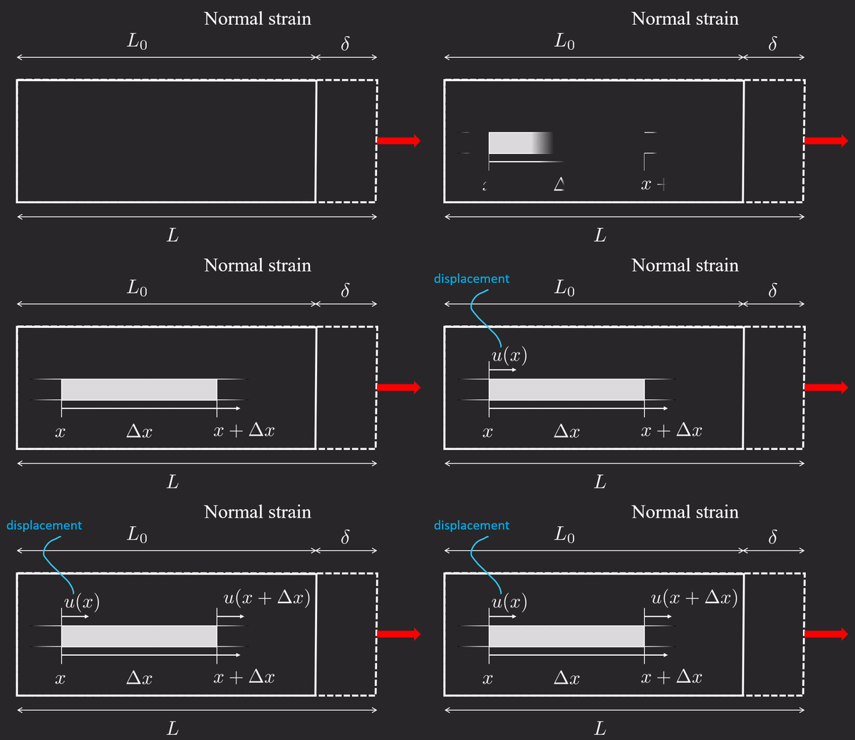
ε : = elongation original length = u ( x + Δ x ) − u ( x ) Δ x → d u d x = ε \varepsilon :=\dfrac{\textrm{elongation} }{\textrm{original}\;\textrm{length} }=\dfrac{u\left(x+\Delta x\right)-u\left(x\right)}{\Delta x}\to \boxed{\dfrac{d\;u}{d\;x}=\varepsilon} ε := original length elongation = Δ x u ( x + Δ x ) − u ( x ) → d x d u = ε
⚠ Note
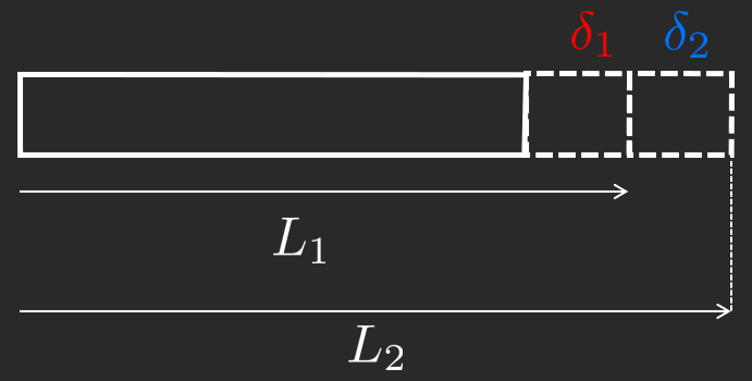
Note that engineering strain cannot be added:
ε = δ 1 + δ 2 L 1 ≠ ε 1 + ε 2 = δ 1 L 0 + δ 0 L 0 + δ 1 \varepsilon =\dfrac{\delta_1 +\delta_2 }{L_1 }\not= \varepsilon_1 +\varepsilon_2 =\dfrac{\delta_1 }{L_0 }+\dfrac{\delta_0 }{L_0 +\delta_1 } ε = L 1 δ 1 + δ 2 = ε 1 + ε 2 = L 0 δ 1 + L 0 + δ 1 δ 0 Instead we can use logarithmic strain, which we define as such
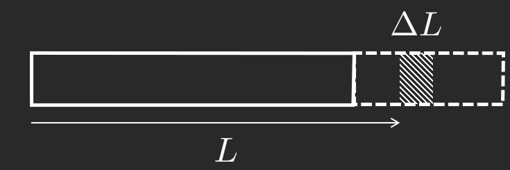
Consider a difference in length, Δ L \Delta L Δ L L L L
Δ ε = Δ L L \Delta \varepsilon =\dfrac{\Delta L}{L} Δ ε = L Δ L if we consider the limit Δ L → 0 \Delta L\to 0 Δ L → 0
lim Δ L → 0 d ε = 1 L d L \lim_{\Delta L\to 0} d\varepsilon =\dfrac{1}{L}d\;L Δ L → 0 lim d ε = L 1 d L Now integrate over the whole length
∫ 0 ε d ε = ∫ L 0 L 1 L d L ⇒ ε L = ln ( L L 0 ) \int_0^{\varepsilon } d\varepsilon =\int_{L_0 }^L \dfrac{1}{L}d\;L\Rightarrow \boxed{\varepsilon_L =\ln \left(\dfrac{L}{L_0 }\right)} ∫ 0 ε d ε = ∫ L 0 L L 1 d L ⇒ ε L = ln ( L 0 L ) this strain can be added.
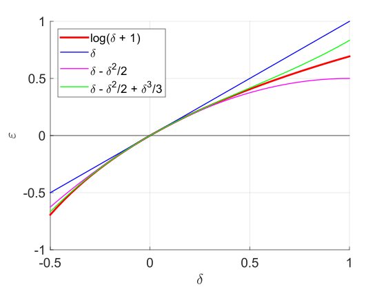
We see especially when δ < < L \delta << L δ << L ε = δ L 0 \varepsilon =\frac{\delta }{L_0 } ε = L 0 δ L = L 0 + δ L=L_0 +\delta L = L 0 + δ δ = 0 \delta =0 δ = 0
clear
syms L_0 delta
taylor(log ( (L_0+delta)/L_0 ), delta, 0 , 'order' , 4 )δ L 0 − δ 2 2 L 0 2 + δ 3 3 L 0 3
\frac{\delta }{L_0 }-\frac{\delta^2 }{2\,{L_0 }^2 }+\frac{\delta^3 }{3\,{L_0 }^3 }
L 0 δ − 2 L 0 2 δ 2 + 3 L 0 3 δ 3 ε L = ln ( L L 0 ) = δ L 0 − δ 2 2 L 0 2 + δ 3 3 L 0 3 − ⋯ \varepsilon_L =\ln \left(\dfrac{L}{L_0 }\right)=\dfrac{\delta }{L_0 }-\dfrac{\delta^2 }{2L_0^2 }+\dfrac{\delta^3 }{3L_0^3 }-\cdots ε L = ln ( L 0 L ) = L 0 δ − 2 L 0 2 δ 2 + 3 L 0 3 δ 3 − ⋯ or
ε L = ln ( L L 0 ) = ε − ε 2 2 + ε 3 3 − ⋯ ⏟ O ( δ n ) where n ≥ 2 \varepsilon_L =\ln \left(\dfrac{L}{L_0 }\right)=\varepsilon \underset{O\left(\delta^n \right)\;\textrm{where}\;n\ge 2}{\underbrace{-\dfrac{\varepsilon^2 }{2}+\dfrac{\varepsilon^3 }{3}-\cdots } } ε L = ln ( L 0 L ) = ε O ( δ n ) where n ≥ 2 − 2 ε 2 + 3 ε 3 − ⋯ Show visualization code
L0 = 1 ;
syms delta
eps1 = taylor(log ( (L0+delta)/L0 ), delta, 0 , 'order' , 2 );
eps2 = taylor(log ( (L0+delta)/L0 ), delta, 0 , 'order' , 3 );
eps3 = taylor(log ( (L0+delta)/L0 ), delta, 0 , 'order' , 4 );
range = [-0.5 ,1 ];
figure ; hold on
fplot(log ((L0+delta)/L0), range,'r' ,'Linewidth' ,2 )
fplot(0 ,range,'-k' ,'HandleVisibility' ,'off' )
fplot(eps1, range,'b' ,'Linewidth' ,1 )
fplot(eps2, range,'m' ,'Linewidth' ,1 )
fplot(eps3, range,'g' ,'Linewidth' ,1 )
xlabel('$\delta$' ,'Interpreter' ,'latex' )
ylabel('$\varepsilon$' ,'Interpreter' ,'latex' )
set(gca,'Fontsize' ,14 )
grid on
legend ('show' ,'location' ,'northwest' )
A rod is compressed from 140mm to 120mm. Determine the linear and logarithmic strain.
We have
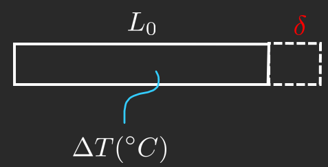
δ = 120 − 140 = − 20 mm \delta =120-140=-20\textrm{mm} δ = 120 − 140 = − 20 mm ε = − 20 140 = − 0 . 142857 \varepsilon =-\dfrac{20}{140}=-0\ldotp 142857 ε = − 140 20 = − 0 . 142857 ε L = ln ( 120 140 ) = − 0 . 154151 \varepsilon_L =\ln \left(\dfrac{120}{140}\right)=-0\ldotp 154151 ε L = ln ( 140 120 ) = − 0 . 154151 Materials can get deformed by heat. The deformation due to head can be modeled using the temperature expansion coefficient, α [ 1 / ° C ] \alpha \;\left\lbrack 1/\degree \mathrm{C}\right\rbrack α [ 1/° C ]
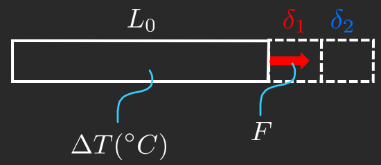
δ = L 0 α Δ T = L 0 ε temp \delta =L_0 \alpha \Delta T=L_0 \varepsilon_{\textrm{temp} } δ = L 0 α Δ T = L 0 ε temp L = L 0 + L 0 α Δ T L=L_0 +L_0 \alpha \Delta T L = L 0 + L 0 α Δ T We can add mechanical strain to thermal strain
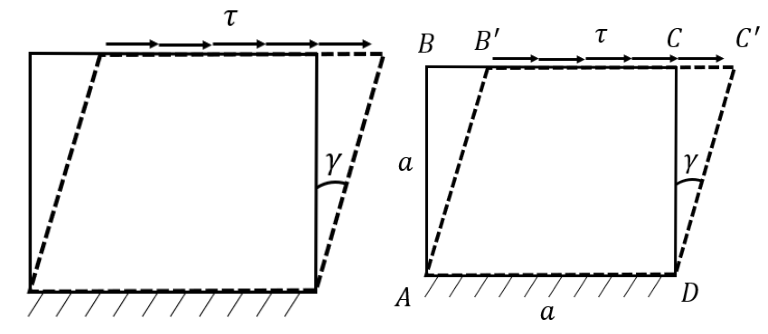
ε tot = ε elast + ε temp \varepsilon_{\textrm{tot} } =\varepsilon_{\textrm{elast} } +\varepsilon_{\textrm{temp} } ε tot = ε elast + ε temp ε tot = σ E + α Δ T \varepsilon_{\textrm{tot} } =\dfrac{\sigma }{E}+\alpha \Delta T ε tot = E σ + α Δ T Strain due to shearing can be modeled by exposing the quad in the figure above to a stress which is horizontal and parallel to its lower edge which is immovable. Then the quad will deform into a parallelogram with the shear angle γ \gamma γ
a 2 = a h cos γ a^2 =a\;h\;\cos \gamma a 2 = a h cos γ where h = A B ′ h=A\;B^{\prime } h = A B ′ γ \gamma γ cos γ ≈ 1 \cos \gamma \approx 1 cos γ ≈ 1 h → a h\to a h → a
γ ≈ tan γ = ∣ B B ′ ∣ a = δ a \boxed{\gamma \approx \tan \gamma } =\dfrac{|B\;B^{\prime } |}{a}=\dfrac{\delta }{a} γ ≈ tan γ = a ∣ B B ′ ∣ = a δ which is analogous to ε = δ / L 0 \varepsilon =\delta /L_0 ε = δ / L 0
The material relation is given by
τ = G γ \boxed{\tau =G\gamma} τ = G γ where G G G it can be shown that
G = E 2 ( 1 + ν ) \boxed{ G=\dfrac{E}{2\left(1+\nu \right)} } G = 2 ( 1 + ν ) E thus the shear modulus is related to the Young's modulus E E E ν \nu ν